
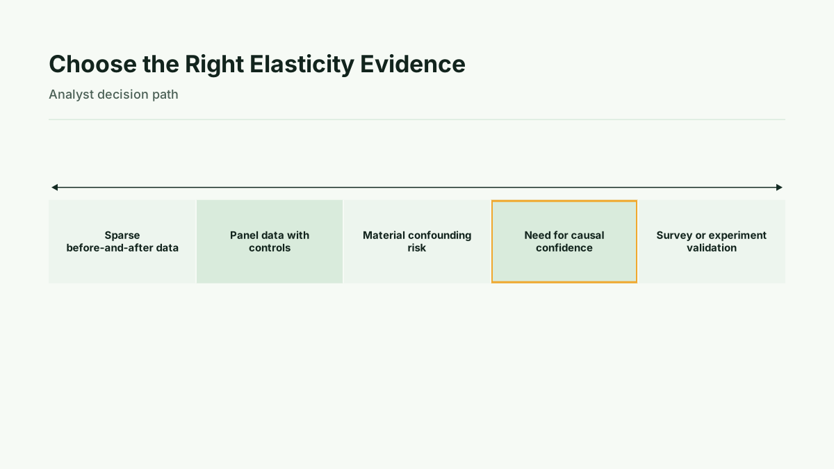
Direct answer: calculate midpoint elasticity immediately when data is sparse, use log-log OLS as the panel-data baseline, escalate to partially linear regression or DoubleML when endogeneity and nonlinear controls matter, and treat the result as decision evidence rather than a permanent demand constant. Before a broad price change, validate the recommendation with stated purchase intent or a randomized price test.
Price elasticity describes the relationship between a change in price and a change in quantity. That relationship can be estimated from observed historical sales, modeled from a regression, simulated for candidate prices, or explored through stated purchase intent. Those are different evidence types. A historical estimate is not the same as a customer saying they would buy, and a modeled revenue result is not an observed outcome.
The decision is therefore not simply “what is the elasticity?” It is “which estimate is credible enough for this pricing decision, and what evidence should come next?”
Start With the Fastest Defensible Calculation
For two observations, midpoint elasticity uses the change in quantity divided by average quantity, divided by the change in price divided by average price. The average price is the mean of the two prices, and the average quantity is the mean of the two quantities. This is suited to a before-and-after price change and avoids choosing one observation as the reference point. See the spreadsheet-ready version of the midpoint formula and the midpoint formula's worked examples.
A spreadsheet should show explicit units in every input: price per subscription per month, units sold per week, or another defined unit of analysis. Do not mix revenue with units sold in the quantity field. The midpoint result is an immediate diagnostic, not proof that price caused the quantity movement.
Point elasticity answers a narrower question: the local response at a particular point on a known or estimated continuous demand curve. It is useful when the curve has been specified, but it requires more structure than a simple two-observation comparison.
With panel data, a log-log demand regression is the baseline model to consider. In that specification, the coefficient on log price is interpreted as price elasticity. The DoubleML elasticity tutorial provides a reference for this modeling context. A log-log coefficient is still an estimate for a defined sample, horizon, product, and specification. It is not a universal constant.
Audit the Data Before Choosing a Model
At minimum, assemble price, units or revenue, timestamp, SKU or market identifier, and a promotion flag. Define the unit of analysis before estimating anything. A weekly SKU-market observation answers a different question from a daily account-level observation.
Plot raw units against raw price for one SKU before transforming variables. The plot can reveal whether there is enough price variation to estimate a relationship and whether a few observations dominate the pattern. Weekly data may smooth daily noise, while daily data may show more immediate responsiveness. The choice is a trade-off between noise and the response horizon you want to study, not a cosmetic formatting decision.
Audit stockouts, missing competitor prices, assortment changes, reporting lags, and promotion timing. Stockouts can make recorded units look like weak demand when the product was unavailable. Promotions can move price and quantity together for reasons unrelated to the ordinary price response. Competitor effects and price endogeneity can also bias an observational estimate. The DoubleML documentation identifies these data and identification concerns.
If a material field is missing, document it rather than silently treating missingness as a neutral value. A sparse before-and-after file may justify midpoint elasticity as a directional diagnostic. It does not automatically justify a causal claim.
Use a Model Ladder That Matches Decision Stakes
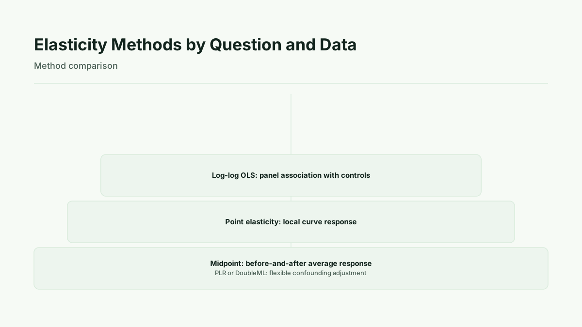
Use the least complex method that can support the decision:
- Midpoint elasticity: a quick before-and-after diagnostic when observations are sparse.
- Point elasticity: a local response estimate when a continuous demand curve is available or estimated.
- Log-log OLS: a panel-data baseline with relevant controls and fixed effects where the data supports them.
- Partially linear regression: an upgrade when the price effect is the focus but controls may have a nonlinear relationship with demand.
- DoubleML: an option when flexible nuisance models, sample splitting, and cross-fitting are warranted. DoubleML uses orthogonalization, sample splitting, and cross-fitting to reduce overfitting bias in flexible nuisance-function estimation. Read the DoubleML method reference.
- Randomized price experiment: the strongest next evidence when the business can assign prices and the decision is material.
The ladder is not a ranking in which the most complex model always wins. More machinery can make assumptions and outputs harder to inspect. Upgrade when confounding, nonlinear controls, or the stakes of a wrong decision justify the additional complexity. Keep the baseline so the incremental value of the upgrade can be evaluated.
Diagnose Endogeneity and Test Whether the Estimate Holds Up
Price can respond to demand signals. If a business raises price when it expects demand to be strong, price may correlate with unobserved demand shocks. In that setting, a price coefficient can describe the historical association without isolating the effect of price.
Use a robustness set rather than one preferred specification. Check placebo periods, holdout validation, clustered standard errors, bootstrap confidence intervals, alternative functional forms, and coefficient stability across control sets. These checks do not turn observational data into an experiment, but they expose sensitivity and unresolved uncertainty.
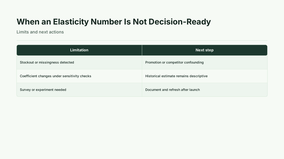
If the estimate changes materially when promotions, competitor measures, fixed effects, or the sample window change, label it descriptive rather than causal. If price variation is weak, a precise-looking coefficient can still be decision-poor. Report the coefficient, confidence interval, data window, model specification, unresolved limitations, and candidate price together.
Translate Elasticity Into Revenue, Margin, and Test Decisions
An absolute elasticity greater than one is commonly described as elastic. An absolute elasticity below one is commonly described as inelastic. The revenue implication depends on the objective and assumptions, as explained by OpenStax on price elasticity. The analyst must identify whether the objective is revenue, unit volume, or margin before recommending a price move.
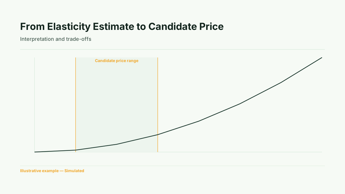
Keep the evidence labels visible. A quantity response calculated from historical sales is observed behavior. A revenue projection under a candidate price is modeled or simulated revenue. A survey response is stated purchase intent. A randomized test result is observed behavior under assigned prices. These should not be merged into a single “expected” number without explaining the distinction.
Use an uncertainty band around any candidate-price simulation and show the time horizon. Short-run and long-run responses can differ, and elasticity should be monitored and refreshed as promotions, competition, seasonality, and market conditions change. DataRobot's guidance on elasticity modeling supports treating elasticity as something to monitor rather than a fixed benchmark.
Add a Second Evidence Stream Before Changing Price
Historical regression and stated-intent research answer different questions. Van Westendorp price range research explores price perception, while Gabor Granger tests stated purchase likelihood at specified price points. Agreement between the modeled elasticity and survey signals can increase confidence. Divergence is useful too: it can indicate that the analyst should investigate the sample, narrow the proposed change, or run a controlled price test.
Kinetic Pricing provides a price range finder, price point tester, feature value ranker, and package and price builder, as well as Kinetic Pro scenario research for a second evidence stream. These methods provide research evidence and scenario modeling, not claimed observed customer outcomes. See the overview of price perception surveys and Kinetic Pro.
Method
Define the objective and metric first. Select the sample window and unit of analysis. Audit the data and engineer controls for promotions, timing, identifiers, and other available demand factors. Estimate midpoint elasticity for an immediate diagnostic, then fit log-log OLS as the panel-data baseline. Escalate to partially linear regression or DoubleML when confounding and flexible controls justify it. Validate with robustness checks, document the estimate, simulate candidate revenue or margin outcomes with explicit labels, and compare the result with stated purchase intent or a randomized experiment. The evidence base for this process includes OpenStax, the DoubleML tutorial, DataRobot guidance, Economics Help, Omni Calculator, and the supplied Kinetic Pricing product information.
Interpretation
Interpret elasticity as evidence about a defined product or market unit, data window, time horizon, and objective. State whether each finding is correlational, modeled, simulated, based on stated intent, or based on observed experimental behavior. Monitor the estimate as conditions change. A coefficient near a benchmark is contextual evidence, not a universal target.
Limits
Observational price endogeneity, stockouts, omitted promotions, assortment shifts, competitor shocks, weak price variation, model misspecification, and short-run versus long-run differences can limit interpretation. Surveys can contain hypothetical bias. Revenue simulations carry uncertainty. No single historical estimate guarantees future behavior, and a more complex model does not automatically remove every limitation.
Next step
Pull the latest price and quantity history. Calculate midpoint elasticity with explicit price and quantity units. Classify the data as sparse or panel-ready, audit confounders, choose the lowest-complexity credible method, and report uncertainty. If the decision is material or the estimate is unstable, obtain a second evidence point through Kinetic Pricing research or run a controlled price test before a broad change. Compare the modeled result with a Kinetic Pro study.
Additional context on these methods is available from 1%, DoubleML's elasticity tutorial, 30%, absolute elasticity greater than 1 means demand is elastic, full plans page, Price elasticity of demand and price elasticity of supply | OpenStax, Estimation of Price Elasticities with Double/Debiased Machine Learning (DoubleML tutorial) and Price elasticity of demand modeling: DataRobot docs.
Run this method with your users
Start 30-day free trial to run every method with your users, or Buy one study when one decision needs evidence now.
Sources
OpenStax, Price elasticity of demand and price elasticity of supply
DoubleML, Estimation of Price Elasticities with Double/Debiased Machine Learning
DataRobot, Price elasticity of demand modeling
Omni Calculator, Price elasticity of demand
Economics Help, Calculating price elasticity of demand
Kinetic Pricing, Van Westendorp pricing research for SaaS
Kinetic Pricing, Kinetic Pro
Kinetic Pricing, Pricing plans